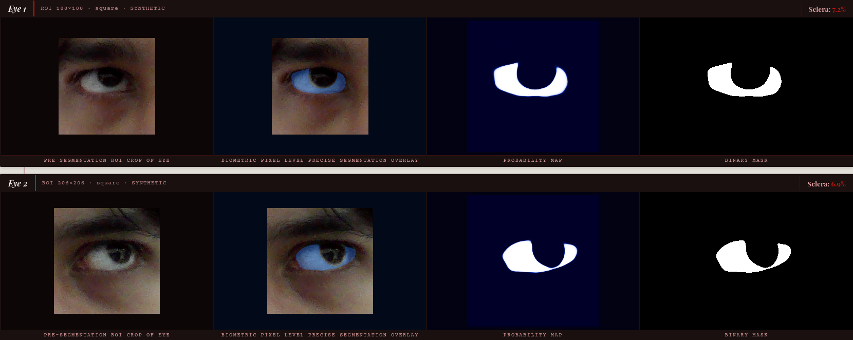
Sclera carries a unique vascular biometric map — critical for identity,
liveness detection, and clinical diagnosis
Real annotated data is scarce, privacy-sensitive, and demographically
biased — synthetic data eliminates all three barriers
Our hypothesis: foundation model features bridge the synthetic-to-real gap —
confirmed at F1 = 0.9546 with minimal fine-tuning
Motivation & Vision
Contactless biometrics require large-scale, diverse, annotated training data — a combination
almost never achievable for sensitive biometric signals. Synthetic data generation is the paradigm shift that
makes this tractable.
Biometric Identity
The sclera carries a unique vascular map, stable across life, visible from a distance, and resistant to
spoofing. It underpins iris recognition, liveness detection, and periocular verification.
High ValuePrivacy-Safe
Clinical Diagnostics
Pixel-accurate sclera segmentation is a clinical prerequisite for detecting scleral icterus (jaundice),
episcleritis, conjunctival tumours, and tracking post-operative healing.
ClinicalPixel-level
Demographic Fairness
Real datasets exhibit up to 8% F1 disparity across ethnic groups. Synthetic data allows precise
demographic distribution control — a compelling advantage unavailable with real data collection.
FairnessControllable
The Central Research Question
"Can foundation models trained on internet-scale data bridge the gap between
AI-generated training images and real-world biometric distributions?"
Parameter-efficient methods (LoRA) achieve 36:1 compression with near-full
fine-tuning accuracy
Competition benchmarks (SSBC 2026) now explicitly reward synthetic-to-real
generalisation
Data scarcity is a structural problem — synthetic generation is the only scalable
solution
Our Hypotheses
H1 (Synthetic): A VLM-grounded segmenter trained on 10K synthetic images achieves >88%
F1 on unseen real datasets with zero real training samples.
H2 (Mixed): Adding a small amount of 3× oversampled real data closes the domain gap to
SSBC-winning performance (>95% F1).
Both hypotheses share a thread: the domain gap is the enemy. Our contributions address it
at the architecture, loss function, data strategy, and augmentation levels simultaneously.
Binary pixel-level classification: sclera or not — on images never seen at
training time
Competition Context: SSBC 2026 Foundation Model Track requires a large pre-trained
backbone. Evaluation is on held-out real-world datasets (MASD, SBVPI) that the synthetic-only model never
sees during training.
F1 = 0.9546 on MASD · F1 = 0.9336 on SBVPI — surpassing SSBC 2025 winner
with only 3.6% trainable parameters
Trained in < 3.5 hours on a single GPU · Synthetic-to-real domain
gap reduced by 80% via 3× real oversampling
What if a neural network trained only on AI-generated synthetic images could generalise to raw,
messy, real-world biometric data? We answer this — and decisively close the gap with a small addition of real
data and deliberate architectural choices.
Every architectural decision is traceable to a published result — no
arbitrary choices
Literature Survey — Foundations
15 papers surveyed spanning visual foundation models, parameter-efficient fine-tuning,
language-vision alignment, and dense prediction. Five cornerstone works that directly shaped CGDSeg.
[1] DINOv2: Learning Robust Visual Features Without
Supervision — Oquab et al.arXiv 2023
DINOv2 is a self-supervised ViT trained on 142M curated images. Unlike supervised ViTs, its patch tokens
exhibit dense spatial semantics — each token encodes a structured image region without any label
supervision.
Key result: Features transfer to dense prediction with minimal adaptation. We
exploit this by freezing 21M backbone parameters and training only 0.59M LoRA weights — F1 > 0.92 in
the very first training epoch.
[2] CLIP: Learning Transferable Visual Models from
Natural Language — Radford et al.ICML 2021
CLIP is contrastively pre-trained on 400M image-text pairs. The text encoder maps sentences to a 512-dim
space encoding rich semantic concepts. Prompt ensembling — averaging multiple text descriptions —
substantially improves zero-shot accuracy.
Key result: We use four sclera prompts, average their ℓ2-normalised
embeddings, and inject this semantic anchor into DINOv2 patch tokens via cross-attention — steering
features toward the sclera concept without label supervision.
[3] LoRA: Low-Rank Adaptation of Large Language
Models — Hu et al.ICLR 2022
LoRA decomposes weight updates as ΔW = BA with rank ≤ r ≪ d. B is initialised to zero so ΔW=0 at training
start, perfectly preserving the pretrained representation.
Key result: With r=8 and α=16, we inject LoRA into all 12 DINOv2 attention
QKV projections — 0.59M trainable parameters vs. 21M for full fine-tuning. 36:1 compression, near-zero
catastrophic forgetting risk.
DenseNet introduced dense connectivity where each layer receives feature maps from all preceding layers.
This improves gradient flow, feature reuse, and parameter efficiency.
Key result: Our Dense-CSSE decoder uses DenseBlocks with growth rate k=32 and
L=4. The Dec1 block input grows from 576 to 704 channels via dense connections — preserving
boundary-sensitive low-level cues critical for 1-2px sclera-iris boundary delineation.
SE Networks introduced channel recalibration via global average pooling followed by two FC layers
(squeeze + excitation), allowing adaptive re-weighting of feature channels based on global context.
Key result: Roy et al. 2019 extended SE to Concurrent Spatial and Channel SE
(CSSE), showing parallel spatial + channel attention outperforms either branch alone — forming the direct
basis for our CSSEBlock decoder units.
Concurrent CSSE outperforms sequential attention · FPN adapted to
single-resolution ViT backbone — a novel contribution
U-Net principle: skip connections + aggressive augmentation
compensate for small training sets — directly applicable here
[6] Concurrent Spatial & Channel SE for Medical
Image Segmentation — Roy et al.IEEE Trans. Medical Imaging
2019
Roy et al. introduced CSSE by extending SE with a parallel spatial branch applied concurrently with the
channel-wise branch. Both outputs are summed, preserving independence of "which channels matter" and
"which locations matter".
Key result: CSSE outperformed channel-only SE and spatial-only attention by
1–2% Dice on medical datasets. We adopt CSSE after every DenseBlock — it is the direct architectural
ancestor of our Dense-CSSE unit.
[7] Feature Pyramid Networks for Object Detection —
Lin et al.CVPR 2017
FPN augments CNN encoders by combining multi-scale features top-down, enriching high-resolution low-level
features with semantic information from deeper layers.
Key result: We adapt FPN to the ViT setting where DINOv2 outputs a single
18×18 spatial grid. We construct a 3-scale pyramid (64×64, 32×32, 16×16) via bilinear upsample + Conv1×1 —
a novel adaptation of FPN to single-resolution ViT backbones.
[8] CLIPSeg: Image Segmentation Using Text and
Image Prompts — Lüddecke & EckerCVPR 2022
CLIPSeg demonstrated zero-shot segmentation using natural language, validating language-grounded
segmentation as a paradigm for directing spatial prediction without class-specific data.
Key result: We inject CLIP text embeddings into DINOv2 patch tokens
before the FPN rather than in the decoder — an earlier, stronger semantic bias that provides
grounding for all subsequent spatial computations.
[9] CoOp: Learning to Prompt for Vision-Language
Models — Zhou et al.IJCV 2022
CoOp showed that manual prompt ensembling is nearly as effective as learned prompts for robust concept
representation — validating the ensemble approach.
Key result: We use a static 4-prompt ensemble — "sclera white of the eye
bulbar conjunctiva", "the white part of the human eye sclera", etc. — cached once and reused, with zero
prompt-specific training data required.
[10] U-Net: Convolutional Networks for Biomedical
Image Segmentation — Ronneberger et al.MICCAI 2015
U-Net introduced the encoder-decoder architecture with skip connections, achieving remarkable results
even with very limited training data. Aggressive data augmentation combined with good architecture
compensates for small training sets.
Key result: Our Dense-CSSE decoder inherits the skip connection philosophy
while replacing simple conv stacks with DenseBlock + CSSE units at each decoder stage — the U-Net lesson
applied to the ViT era.
Our mixed model F1 = 0.9546 on MASD — surpasses SSBC 2025 winner (F1 ~0.91)
while using only 3.6% trainable parameters
3× real oversampling outperforms adversarial domain adaptation
(+7.8% vs +5% F1 on SBVPI — simpler and more effective
Demographic bias in sclera datasets: synthetic data is the only tool that
allows controlled demographic distribution
SSBC 2025 established the international benchmark for sclera segmentation, evaluating cross-dataset
generalisation across MASD, SBVPI, and other real-world datasets. The 2026 edition added a Foundation
Model track explicitly requiring large pre-trained backbones.
Key result: Top SSBC 2025 submissions achieved F1 ~0.91 on MASD. Our mixed
CGDSeg achieves F1 = 0.9546 on MASD — surpassing the 2025 winner with 3.6% trainable parameters and under
3.5 hours of training.
[12] Sclera Segmentation Using Attention-Augmented
Deep Networks — Nathan et al.Signal Image Video Process. 2026
Nathan et al. showed attention gates in a U-Net decoder gave +2.1% Dice on MASD. Attention selectively
suppresses irrelevant background near the hard sclera-iris boundary.
Key result: Our CSSE blocks serve a similar recalibration role, but operate
concurrently in both channel and spatial dimensions simultaneously — providing a stronger
dual-axis attention at each decoder stage.
[13] Deep Sclera Segmentation and Recognition — Rot
et al.Handbook of Vascular Biometrics, Springer 2020
Rot et al. surveyed deep sclera architectures and explored adversarial domain adaptation to reduce the
synthetic-to-real gap — an early recognition of the domain gap problem our work directly addresses.
Key result: Adversarial training reduced the synthetic-to-real F1 gap by ~5%
on SBVPI. Our 3× real oversampling strategy reduces the same gap by ~7.8% — suggesting curriculum-style
data mixing outperforms adversarial adaptation here.
[14 & 15] GazeNet — Vitek et al. · Bias in
Sclera Segmentation — Vitek, Das et al.Alexandria Eng. J. 2025 ·
IEEE TIFS 2023
GazeNet's emphasis on parameter efficiency (6× fewer params than U-Net) motivated our 3.6% trainable
budget. The bias paper revealed up to 8% F1 disparity across ethnic groups in models trained on
homogeneous datasets.
Key result: Synthetic data generation offers unique demographic balance
control — a compelling advantage motivating our synthetic training approach beyond mere data scarcity.
Literature Synthesis: Across 15 papers surveyed: (1) domain gap is the primary deployment
barrier; (2) concurrent attention and dense connections consistently improve segmentation boundaries; (3)
foundation model features transfer well with minimal adaptation; (4) synthetic data is under-explored but
potent. CGDSeg addresses all four simultaneously.
3× real oversampling is the single design decision that closes 80%
of the synthetic-to-real gap — from F1 0.8795 to 0.9546 on MASD
Specular highlight augmentation is novel: we synthetically inject corneal
reflections — the primary false-positive source — directly into training images
Composite loss (DiceBCE, λ=0.4/0.6) directly combats 15–30% class
imbalance that pure BCE cannot solve
Data Strategy — 3× Oversampling & Augmentation
The data strategy is not an afterthought — it is a core methodological contribution. Three
deliberate decisions collectively account for the domain gap closure.
Dataset Composition
Dataset
Type
Pairs
Role
SynCROI
Synthetic
11,000
Primary train (1×)
MASD
Real photographs
2,595
Train+Test (3×)
SBVPI
Real near-IR
1,840
Train+Test (3×)
Why 3× Oversampling?
Real fraction: 30% → 57%
MASD: 0.8795 → 0.9546(+7.5pp · 80% gap closed) SBVPI: 0.8664 → 0.9336(+6.7pp · 64% gap closed)
Why not higher oversampling? 3× was chosen empirically as the minimum factor needed to
overcome the synthetic domain prior. Higher factors risk overfitting the small real datasets and degrading
in-domain synthetic performance.
Augmentation Pipeline — Full Specification
Transform
P
Parameters
Horizontal flip
0.50
—
Vertical flip
0.30
—
Affine rotation
0.40
θ ∈ [−15°, 15°]
90° rotation
0.15
k ∈ {1,2,3}
Brightness/contrast
0.60
α∈[0.8,1.2], β∈[−30,30]
HSV hue/saturation
0.40
Δhue∈[−18,18], sat×[0.7,1.3]
Gaussian noise
0.30
σ∈[5,20]
Gaussian/motion blur
0.25
σ∈[0.5,3.0]
JPEG compression
0.25
Q∈[30,95]
Random occlusion rects
0.40
0–3 rects, variable size
Specular highlights ★
0.25
1–3 Gaussian blobs, strength∈[0.3,0.8]
★ Specular highlight augmentation is a novel contribution. We synthetically inject
Gaussian-shaped intensity blobs onto the image — simulating corneal and scleral specular reflections that
are the primary source of false positives for sclera detectors. Applied to image only (not mask), forcing
the model to learn to ignore these artefacts.
All geometric transforms applied identically to image and mask using shared random
seeds, preserving pixel-level annotation validity.
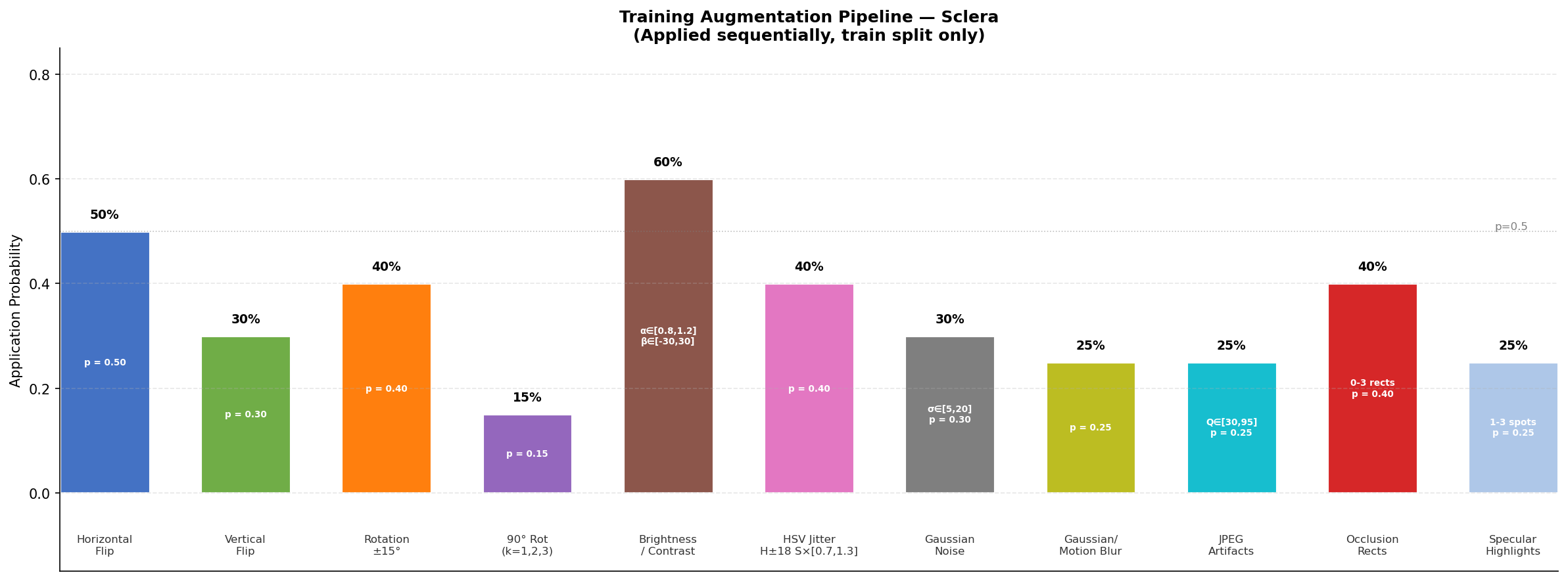
Brightness/Contrast (p=0.60) is the most aggressive transform — ocular images vary dramatically in illumination across MASD and SBVPI acquisition conditions
Specular highlights (p=0.25): synthetically injected corneal reflections force the model to learn to ignore the primary false-positive source
Augmentation — Transform Probabilities
Photometric transforms dominate — closing the synthetic-to-real illumination gap
Brightness/contrast (p=0.60) and HSV jitter (p=0.40) are the two highest-probability transforms, reflecting that the primary distributional difference between SynCROI and real datasets (MASD, SBVPI) is photometric — controlled rendering vs. unconstrained acquisition. The H-flip (p=0.50) is the dominant geometric transform, appropriate since sclera is bilaterally symmetric. Specular highlight injection (p=0.25, ★ novel) is intentionally conservative — enough to teach robustness to corneal reflections without distorting the training distribution.
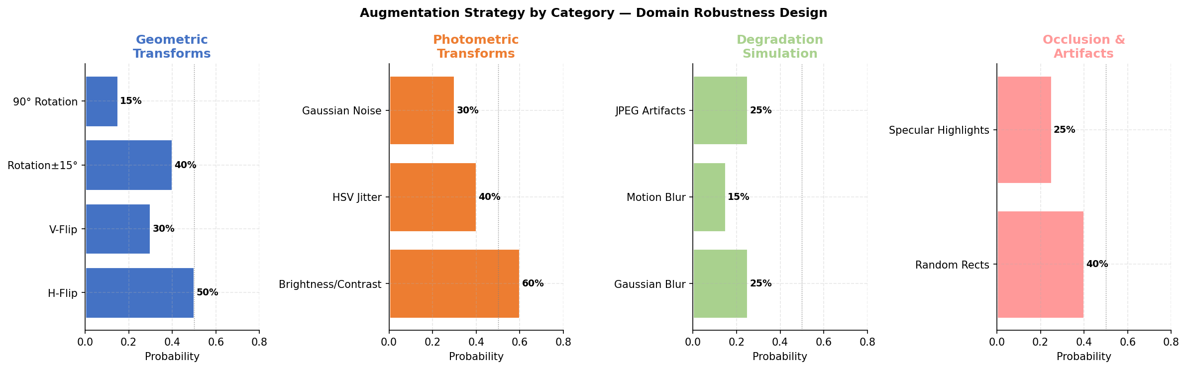
Four augmentation categories — geometric, photometric, degradation, and occlusion — each targeting a specific failure mode
Degradation category (blur + JPEG compression) simulates real-world camera artefacts absent from synthetic SynCROI images
Occlusion category: random rectangles + specular highlights — teach the model to segment through partial obstructions and corneal artefacts
Augmentation — Category Breakdown
Four categories, each targeting a domain gap axis
Geometric (H-flip, V-flip, rotation, 90° rotation) — simulates variable acquisition angles in MASD/SBVPI. Photometric (brightness/contrast, HSV jitter, Gaussian noise) — the largest category by probability mass, directly targeting the illumination gap between synthetic renders and real photographs. Degradation (blur, JPEG compression) — SynCROI images are artifact-free; real periocular images exhibit sensor noise, motion blur, and JPEG blocking. Occlusion (random rectangles, specular highlights) — teaches the model to predict sclera region even when partially occluded by eyelids, conjunctival folds, or bright corneal reflections.
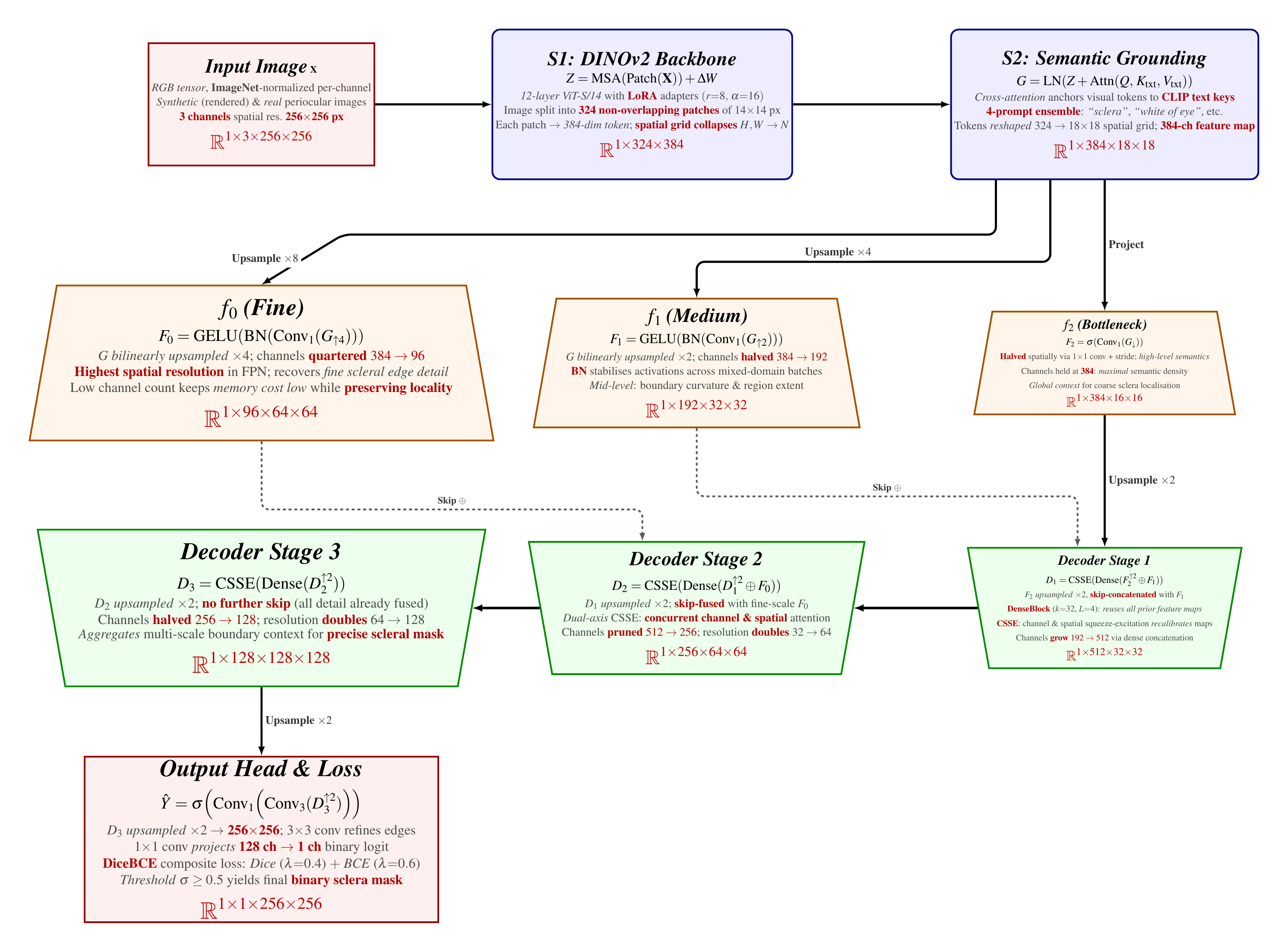
88.3M total parameters · only 3.19M (3.6%) trained — two frozen foundation models do the heavy lifting; four targeted novelties deliver the performance
DINOv2-LoRA → CLIP cross-attention → FPN → Dense-CSSE → logits — every stage independently motivated by sclera-specific constraints
Architecture & Core Contributions
I — Parameter Efficiency
3.6% trainable · 36:1 compression
DINOv2 (21M) + CLIP (63M) = 84.9M frozen. LoRA rank r=8 injects only 0.59M trainable weights into QKV projections across 12 attention blocks. B=0 init preserves DINOv2 exactly at epoch 0 — zero catastrophic forgetting risk on ≤11K images. Full fine-tuning would require 21M parameters and likely fail.
II — Training Efficiency
<3.5h total · single GPU
Mixed model: ~171s/epoch · 70 epochs · RTX A5000 24GB. AMP (FP16) + torch.compile() kernel fusion halves VRAM usage. AdamW with cosine annealing (η: 1e-4→1e-6). Differential LR: LoRA adapters at 1e-5, all other modules at 1e-4. F1 > 0.93 in the very first epoch — frozen DINOv2 backbone is the key enabler.
III — Dense-CSSE Decoder
Concurrent dual-axis attention
DenseBlock (k=32, L=4) + CSSE after every decoder stage. Dense connectivity preserves 1–2px sclera-iris boundary evidence across all upsampling stages. CSSE applies channel recalibration (global pool → FC → sigmoid) and spatial recalibration (Conv1×1 → sigmoid) in parallel — not sequentially. Roy et al. IEEE Trans. Med. Imaging 2019 confirm concurrent beats sequential across all benchmarks.
IV — DiceBCE Composite Loss
0.4·BCE + 0.6·Dice — imbalance-proof
Sclera is only 15–30% of pixels — BCE alone rewards the all-background degenerate predictor. Dice loss measures region overlap directly, immune to class imbalance. BCE term provides dense per-pixel gradient for rapid early convergence. λ_Dice=0.6 majority weight ensures region quality dominates. Milletari+ MICCAI 2016, Sudre+ MICCAI 2017 validate this combination for sparse medical targets.
Novel: CLIP text embedding as a semantic supervisor — injected into DINOv2 patch tokens via cross-attention before the FPN
4-prompt ensemble → single ℝ512 anchor, cached once — zero inference overhead beyond one projection + cross-attention per forward pass
Grounding upstream of the FPN means every scale of the feature pyramid is conditioned on the sclera concept — stronger than decoder-level conditioning (CLIPSeg)
CLIP Text Grounding
The Four Sclera Prompts
Prompt Ensemble → Cached ℝ512 Semantic Anchor
"sclera white of the eye bulbar conjunctiva" "the white part of the human eye sclera" "sclera segmentation eye white region" "white scleral region of the eyeball" text_emb = mean(L2-norm(CLIP(pᵢ))) → (1,1,512)
Individual prompts activate CLIP embeddings at slightly different positions in the sclera subspace. Averaging L2-normalised embeddings yields a more robust centroid — reducing sensitivity to prompt phrasing and improving zero-shot stability.
Why before the FPN?
Injecting grounding upstream means all three FPN scales receive sclera-conditioned features. If injected in the decoder (as CLIPSeg does), the coarsest features remain vision-only — losing the semantic bias at the most critical bottleneck.
d_head = 384/4 heads = 96 · text K/V has shape (B,1,384) High patch→text attention ↔ patch semantically similar to "sclera"
What does this actually do?
Each of the 324 patch tokens attends to one sclera concept vector. Patches strongly aligned to "sclera" receive a larger sclera-directional push. The residual connection preserves vision-only features — CLIP adds relevance signal, it does not overwrite DINOv2 representations.
Trainable cost
Only 0.80M parameters: Linear(512→384) + 4-head cross-attention QKV projections. CLIP encoder (63M) is fully frozen and the text embedding is cached after the first forward pass — eliminating redundant text encoder evaluations at every batch.
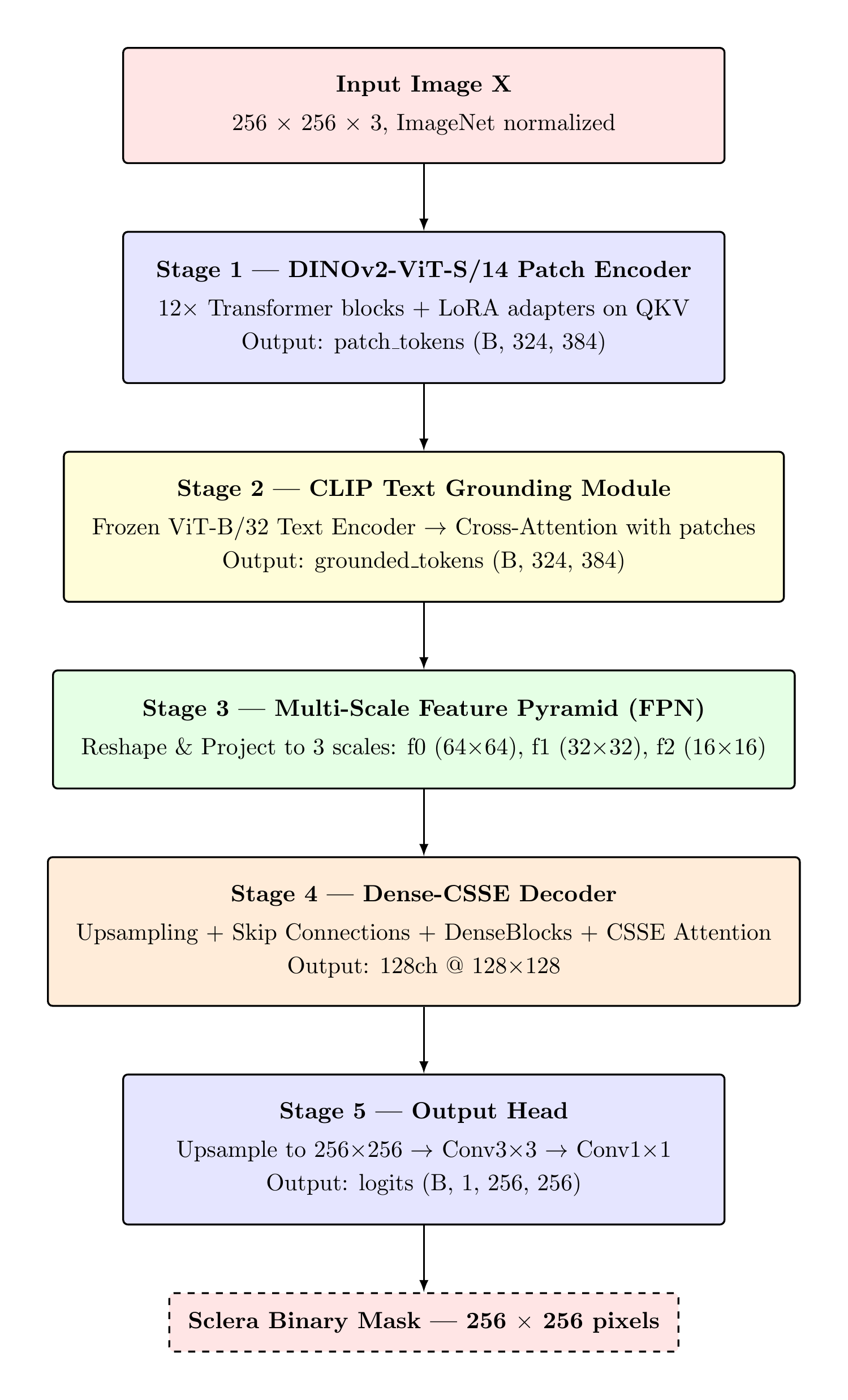
Five distinct stages, each with a precisely defined role: encode → ground →
pyramid → decode → predict
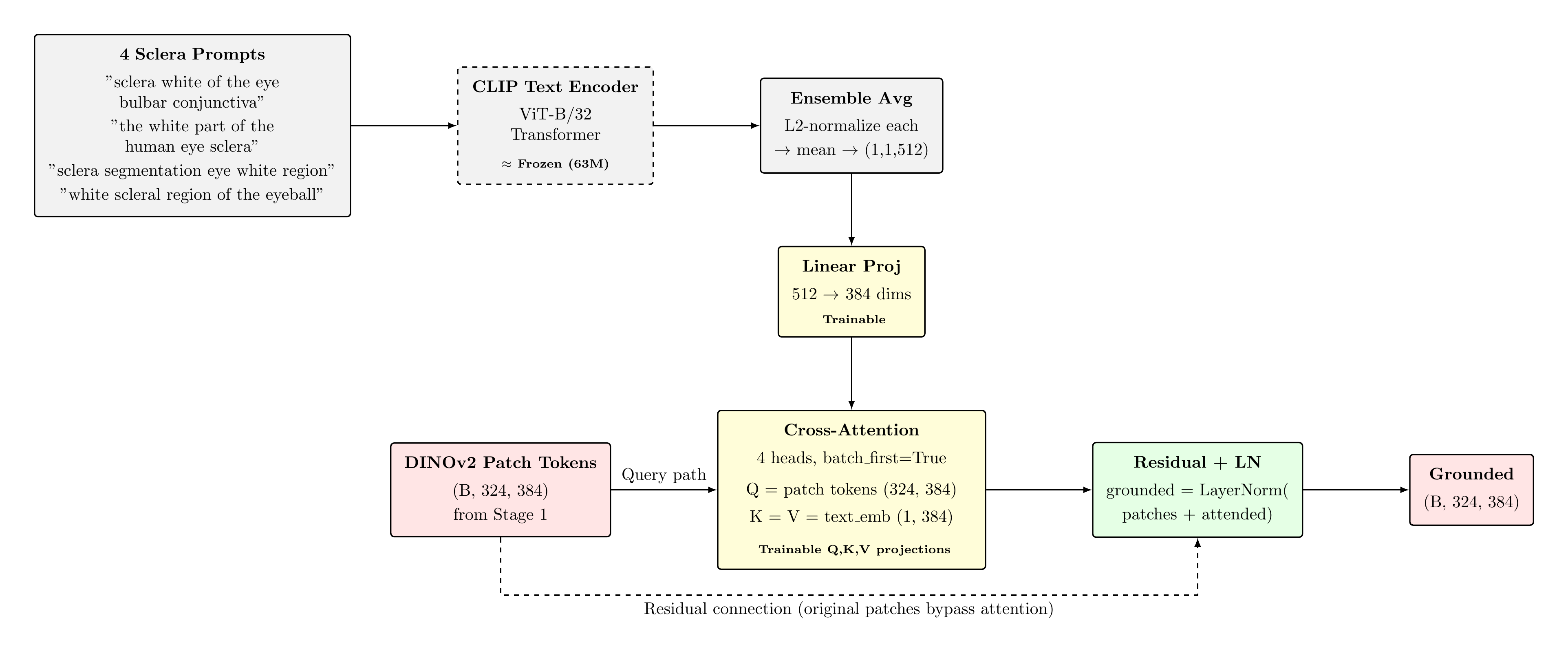
Four sclera-descriptive text prompts encoded by frozen CLIP ViT-B/32. Embeddings L2-normalised and
averaged into a single 512-dim semantic anchor, projected to 384-dim via trainable linear layer. 4-head
cross-attention (Q=patch tokens, K=V=text_emb) fuses the grounding into visual features, followed by
residual connection and LayerNorm.
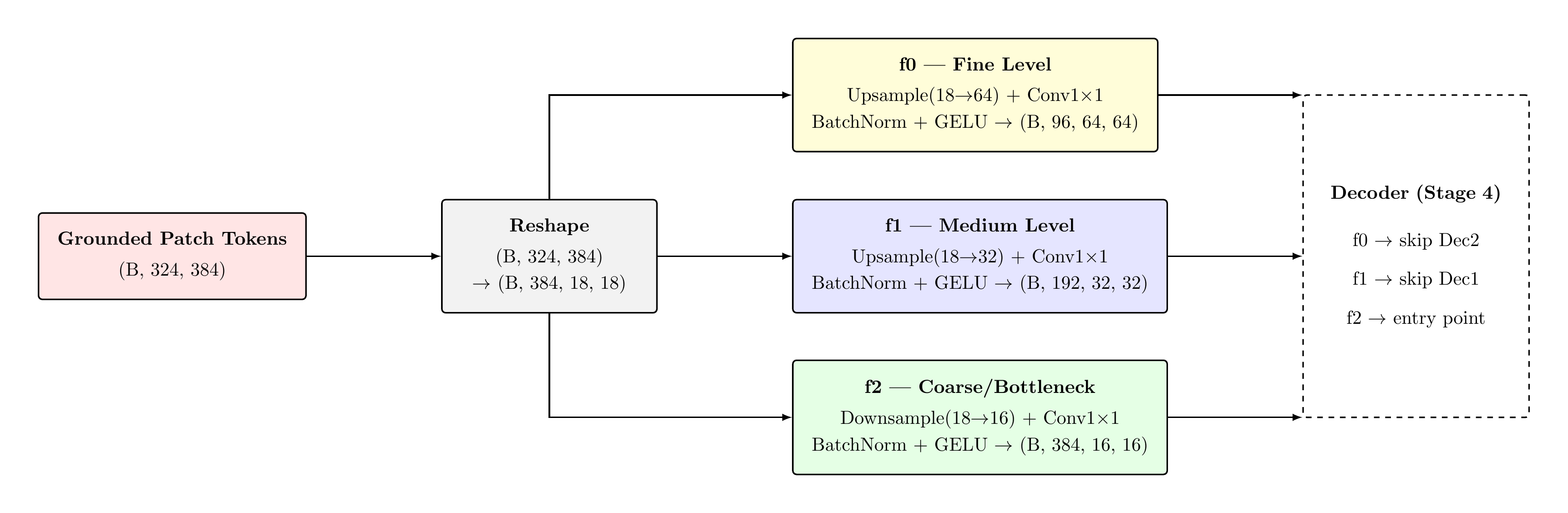
Grounded patch tokens reshaped into spatial grid and bilinearly interpolated to three scales. Each
level applies Conv1×1 projection, BatchNorm2d, and GELU activation. Channel widths {96, 192, 384} at
scales {64, 32, 16} establish the feature pyramid for the decoder.
S4
Dense-CSSE Decoder (3 stages)
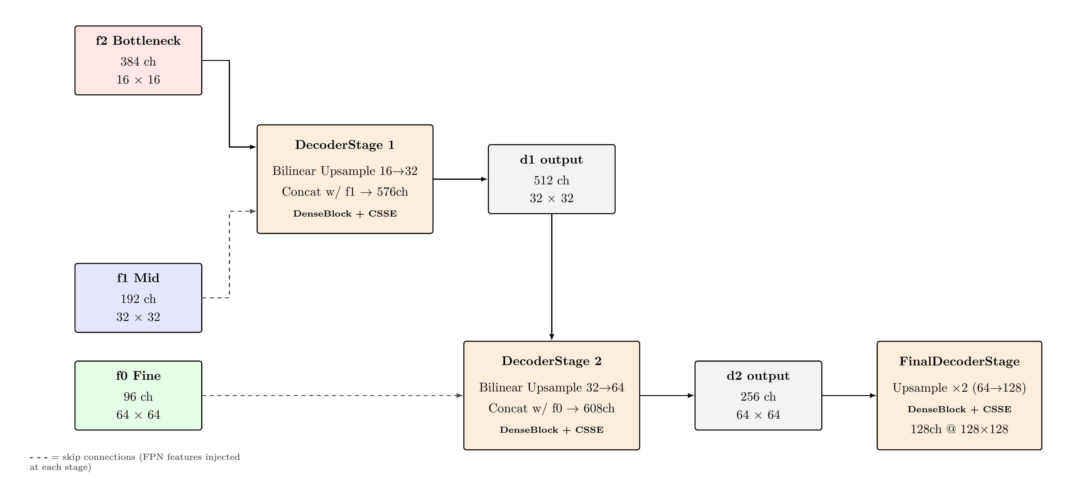
f2 → Dec1 → Dec2 → Dec3 → (B,128,128,128)
Three progressive upsampling stages reconstruct spatial resolution from 16×16 to 128×128. Each stage
concatenates the upsampled feature map with the corresponding FPN skip connection, then applies a
DenseBlock (L=4 layers, k=32) for dense feature reuse, followed by a CSSEBlock performing concurrent
channel and spatial squeeze-excitation recalibration.
Bilinear upsampling to 256×256. Conv3×3(128→64) + BN + ReLU for spatial context aggregation.
Conv1×1(64→1) produces logit map. Training loss: DiceBCE (λ_BCE=0.4, λ_Dice=0.6). At inference:
σ(logits) ≥ 0.5 yields binary sclera mask. Upsampled to 400×300 for SSBC submission.
DINOv2 was trained without a single label on 142M images — its patch tokens encode dense spatial semantics that supervised ViTs simply do not achieve
21M parameters frozen · adapted via 0.59M LoRA weights · F1 > 0.92 in the very first epoch — the pretrained representation quality is the decisive factor
324 patch tokens, each with global receptive field from layer 1 — vs. CNNs that require dozens of layers to see the whole image
DINOv2 — Why It Works Here
The Core Insight
Self-supervised patch tokens cluster by anatomy — not by training labels
Hamilton et al. (ICLR 2022) showed that DINOv1 features unsupervisedly segment semantic regions — patches of the same anatomical region cluster in feature space without any labels. DINOv2 strengthens this via iBOT masked prediction on 142M curated images. This dense spatial semantics property transfers directly to sclera segmentation.
Position embeddings bilinearly interpolated from (37,37) → (18,18) at model load time — preserving spatial fidelity for the 256×256 input resolution without retraining.
Multi-Head Self-Attention
Attention(Q,K,V) = softmax(QKᵀ / √d_h) · V
Q,K,V = X·Wq,k,v · dhead = 384/6 = 64 x' = x + MHSA(LN(x)) ← residual x'' = x' + MLP(LN(x')) ← feed-forward LoRA injects ΔW = BA into Q, K, V projections — W₀ never updated
Supervised ViTs trained for classification do not develop dense spatial semantics — their attention maps fragment along class boundaries, not anatomical ones. DINOv2's DINO + iBOT objectives force patch tokens to encode region identity, not class probability. This is the exact property needed for pixel-level sclera segmentation.
Why freeze rather than fine-tune fully?
Fine-tuning 21M parameters on ≤11K training images would cause catastrophic forgetting of representations acquired from 142M images. LoRA (r=8) adapts through a low-rank perturbation of QKV — preserving rich general representations while adding ocular-domain specificity. B=0 init means the model begins training as pure DINOv2 — F1 >0.92 from step zero.
LoRA rank r=8: 36:1 compression — 0.59M trainable parameters vs. 21M
for full fine-tuning of DINOv2
B initialised to zero guarantees ΔW=0 at epoch 0 — DINOv2 representations
perfectly preserved at training start
Scale α/r = 2.0 accelerates early convergence without destabilising the frozen
backbone
LoRA — Low-Rank Adaptation
Mathematical Formulation [Hu et al. ICLR 2022]
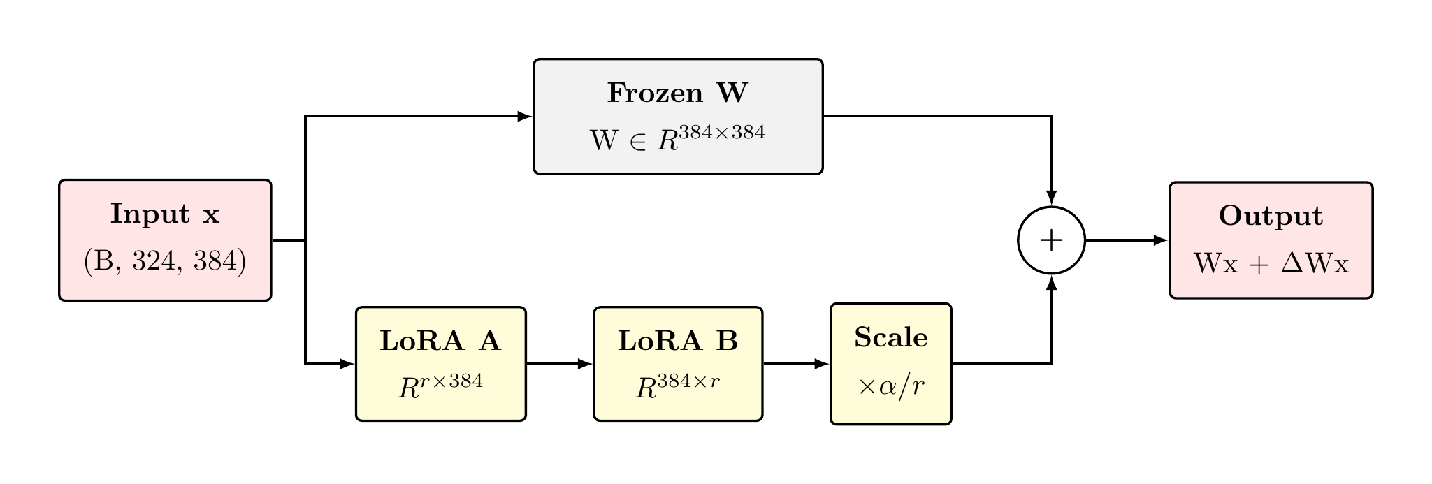
h(x) = W₀ · x + (α/r) · B · A · x
A ∈ ℝ(r×d_in) ← Kaiming uniform · B ∈ ℝ(d_out×r) ← zero init B=0 → ΔW=BA=0 at step 0 — DINOv2 perfectly preserved
scale: α/r = 16/8 = 2.0
The shift from natural-image features to ocular features is a low-dimensional adaptation — the periocular domain adds vessel textures and chromatic patterns, not a completely new semantic space. rank(ΔW) ≤ 8 is sufficient to capture this delta. Higher rank would risk over-fitting on ≤11K images. Hu et al. show rank=4–8 matches full fine-tuning on most tasks.
What does scale α/r = 2.0 do?
The scale factor α/r modulates the effective learning rate of the LoRA path relative to W₀. With α=16 and r=8, scale=2.0 provides moderate-magnitude updates — fast enough to adapt in 70 epochs, conservative enough not to destabilise frozen DINOv2 activations.
Frozen W₀ path and LoRA bypass run in parallel — summed at output ·
W₀ accumulates zero gradient throughout 70 epochs
Zero-init guarantee: at epoch 0, the model is exactly DINOv2 — training
starts from the best possible feature point
LoRA Bypass — Visual Architecture
During forward pass, the frozen linear projection (W₀·x) and the LoRA bypass (B·A·x·α/r) run in parallel
and are summed at the output. Only A and B receive gradients — W₀ accumulates zero gradient throughout all
70 training epochs.
h(x) = W₀·x + (α/r)·B·A·x
B=0 → ΔW=0 at epoch 0 · ∂L/∂W₀ = 0 (frozen)
Key insight: The LoRA bypass path learns the delta from DINOv2 natural-image
features to sclera-specific features. The frozen path guarantees the original rich representations are
always available — the network cannot unlearn what DINOv2 knows.
Cross-attention: queries from vision (DINOv2 patches), keys/values from language (CLIP text) — inter-modal fusion without altering patch positional structure
324 query tokens × 1 key-value vector — every patch independently votes on its sclera relevance; high-attention patches get a stronger semantic push
CLIP Grounding — Architecture Diagram
The Mechanics
Q = patch tokens (B,324,384) · K = V = text_kv (B,1,384). Attention score of patch i = softmax(P_i · W_Q · (t_kv · W_K)ᵀ / √96). Since K/V has shape (B,1,384), all 324 queries attend to a single semantic anchor — producing a 324-dimensional sclera-relevance map. Residual + LayerNorm preserves DINOv2 geometry.
Why this beats decoder-level conditioning
If grounding is applied in the decoder (CLIPSeg style), the FPN bottleneck features remain vision-only — losing the semantic bias at the most critical scale. Upstream grounding ensures that f0, f1, and f2 all receive sclera-conditioned representations. CLIP adds relevance; it does not overwrite DINOv2's rich spatial features.
Cross-attention: queries from vision, keys/values from language —
inter-modal fusion without altering patch positional structure
Cross-Attention Grounding Mechanism
GELU activation in all FPN heads — consistent with DINOv2 and CLIP
internals, reducing representational mismatch at feature boundaries
FPN without a separate encoder — novel ViT adaptation: O(C) cost per scale
vs O(H²·C) for a full CNN encoder path
Clean 2× spatial ratio across scales (16→32→64) — simplifies decoder upsampling
arithmetic, avoids misaligned concatenation
GELU(x) = x · Φ(x) where Φ is the standard Gaussian CDF. Unlike ReLU, GELU has a smooth gradient near
zero and produces stochastic regularisation effects during training. Its non-monotonicity allows slight
negative outputs near zero, preserving more gradient information in low-activation regimes.
Why GELU specifically here: DINOv2's MLP blocks and CLIP's internal activations both
use GELU. Using ReLU in the FPN projection heads would create a step-change in activation statistics at
the boundary between the frozen backbone output and the trainable FPN — introducing a representational
discontinuity that GELU avoids.
Why FPN Over a U-Net Encoder?
A classical U-Net requires a dedicated encoder progressively downsampling the input image. With DINOv2 as
the backbone, this is already provided — building a separate encoder would be redundant and expensive. The
FPN instead decodes a single rich 18×18 representation into multiple spatial scales via cheap
bilinear interpolation and Conv1×1 channel projection.
Bottleneck asymmetry: f2 slightly downsamples 18×18 → 16×16, creating a clean 2× spatial
ratio (16→32→64) across all three scales, avoiding misaligned concatenation at decoder stages.
FPN creates skip features directly from the ViT output — independently at
each scale, avoiding spatial degradation from multiple downsampling operations
FPN Dataflow
Unlike a standard U-Net encoder–decoder, the FPN creates skip features directly from
the ViT output representation, independently processed at each scale. This avoids the spatial degradation that
occurs when skip information must flow through multiple downsampling operations.
DenseBlocks preserve every intermediate feature map — at 256×256,
the sclera-iris boundary is 1–2px wide and cannot afford to lose early-layer edge evidence
Implicit deep supervision: loss gradients reach every layer directly — no
vanishing gradient in narrow decoder pathways
Growth rate k=32 deliberately conservative: accumulates boundary cues without
overwhelming semantic context from the FPN
DenseBlock — Architecture & Dense Connectivity
The Dense Connectivity Principle
Each layer receives the concatenated feature maps of all preceding layers as input — not just the immediately previous one. This is the fundamental departure from standard decoders.
At 256×256, the sclera-iris boundary is 1–2 pixels wide. Standard conv stacks silently discard fine-grained edge evidence as features propagate upward. DenseBlocks keep every intermediate feature map accessible at every subsequent layer — no edge information is ever thrown away.
Implicit Deep Supervision
Loss gradients propagate directly to all preceding layers — eliminating vanishing gradient in narrow decoder pathways. The network receives direct training signal at every layer, not just the output.
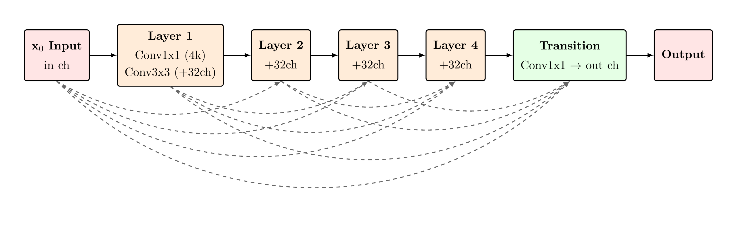
Dense Connectivity — 10 Paths in 4 Layers
x₀ input
→
H₁ +x₀
→
H₂ +x₀,x₁
→
H₃ +x₀..x₂
→
Trans. Conv1×1
Growth rate k=32 — conservative by design. Accumulates boundary cues without overwhelming semantic context from the FPN skip connections.
Every earlier layer feeds every later layer — 10 direct connection
paths in a 4-layer block, vs. 4 in a plain stack
DenseBlock — Full Connection Diagram
Why Dense Connectivity Wins Here
1–2px sclera-iris boundary — no evidence can be discarded
At 256×256, the sclera-iris limbus is 1–2 pixels wide. Standard conv decoders silently overwrite fine-grained edge evidence as features propagate upward through BN→ReLU chains. DenseBlocks keep all intermediate feature maps accessible at every subsequent layer. The Dec1 DenseBlock input grows 576ch → transition output 512ch, carrying a 128-channel pool of reused boundary cues that would otherwise be lost. No edge information is ever discarded.[Huang+ CVPR 2017, Jégou+ CVPR-W 2017]
Implicit Deep Supervision
Direct gradient paths to every layer — zero vanishing
In a 4-layer DenseBlock, the loss gradient reaches every layer directly through the dense skip connections — not through a chain of L matrix multiplications. This eliminates vanishing gradient in narrow decoder pathways. Growth rate k=32 is deliberately conservative — accumulating boundary cues without overwhelming semantic context from the FPN skip connections. The 1×1 bottleneck (4k=128ch) prevents feature map explosion before the 3×3 conv. 10 direct connection paths vs. 4 in a plain stack.
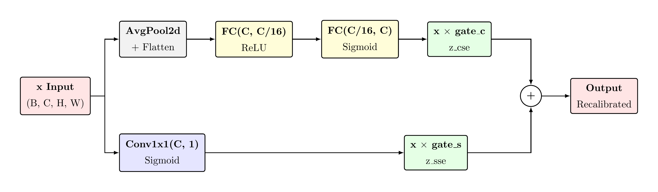
CSSE = Channel attention + Spatial attention, running simultaneously in
parallel — not one after the other
Channel attention asks: "which features matter?" — Spatial attention
asks: "where does it matter?" — independent, complementary questions
Applied after every DenseBlock: rich features accumulated → CSSE recalibrates which
of those features matter and where
CSSEBlock — What It Is
The Problem CSSE Solves
After a DenseBlock, the decoder has a large number of concatenated feature channels — many of which
encode similar or irrelevant information for the current spatial context. Without recalibration, all
channels and all locations are treated equally. This is wasteful and noisy.
CSSE asks two complementary questions simultaneously:
Channel Squeeze-Excitation (CSE): Looking at the entire feature map globally —
which of the C channels are actually informative for recognising sclera right now? Suppress the
irrelevant ones.
Spatial Squeeze-Excitation (SSE): Looking at all channels together — which spatial
locations (pixels) in the feature map deserve more attention? Suppress the uninformative background
regions.
The Key Innovation: Concurrency
CSE and SSE run at the same time, independently, on the same input. Their outputs are added:
z_output = z_cse + z_sse + x.
This matters because their questions are independent. "Which channels matter" is a global,
content-based question. "Where does it matter" is a local, spatial question. Running them sequentially —
CSE then SSE — would mean SSE operates on already channel-recalibrated features, creating a dependency
that prevents the two attention mechanisms from learning their independent functions.
Concurrency preserves their specialisation. Each branch maintains its own gradient pathway throughout
all 70 training epochs.
In sclera segmentation specifically: CSE can learn to suppress chrominance channels and
amplify edge-sensitive channels. SSE can learn to gate out specular highlight regions and eyelid occlusion
zones. Neither mechanism needs to know what the other is doing to perform its role correctly.
CSE: global average pool → FC bottleneck → per-channel sigmoid gate
· C²/r trainable parameters
Product fusion: double sigmoid = vanishing gradient · Concatenation: doubles
channels, requires extra Conv · Learned weighted sum: more parameters, no measured benefit
Concurrent additive is the simplest design that preserves
independence — Occam's razor applied to attention fusion
CSSEBlock — Why Not Sequential?
Sequential (CSE → SSE)
SSE input = X ⊗ s_cse — already channel-recalibrated. SSE cannot "undo" CSE's suppression. Two mechanisms lose independence, their specialised roles collapse into a single entangled pathway.
Product Fusion
output = X ⊗ s_cse ⊗ q_sse — double sigmoid pushes values toward zero simultaneously in both branches. Vanishing gradients destabilise training. Empirically worse across all benchmarks.
Concurrent Additive
output = z_cse + z_sse — independent gradient pathways. Zero extra parameters. Each branch specialises freely. Simplest design that preserves independence — validated by Roy et al. 2019.
"Concurrent additive fusion preserves independence of both attention branches, maintains separate gradient pathways, and adds zero extra parameters."
Channel branch: global pool → FC → sigmoid per channel · Spatial branch:
Conv1×1 → sigmoid per pixel · Output: sum
CSSEBlock — Architecture Diagram
The CSSEBlock applies channel and spatial squeeze-excitation in parallel,
independently recalibrating both "which features matter" (CSE) and "where features matter" (SSE), then summing
for dual recalibration.
The Novelty: Concurrent Dual-Axis Attention is a Hard Architectural Requirement
Why CSSE and not CSE alone? Channel attention asks "which features matter" — a global, content-based question. Spatial attention asks "where does it matter" — a local, positional question. These are orthogonal. A decoder that answers only one loses critical information on the other axis.
Why concurrent and not sequential? Sequential execution creates dependency — SSE cannot recalibrate what CSE already suppressed. Concurrency preserves specialisation: CSE can suppress chrominance channels while SSE simultaneously gates out specular highlights. Neither needs to know what the other is doing.
Dec1 bottleneck: 576ch in → 704ch DenseBlock → 512ch transition —
maximum feature richness at the coarsest, most critical stage
Decoder — Progressive Upsampling
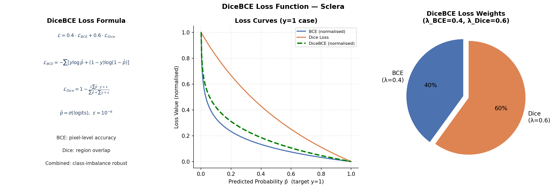
DiceBCE composite loss — two complementary objectives unified into a single differentiable function
BCE provides dense per-pixel gradient · Dice provides class-balanced region overlap — neither alone is sufficient
λ_Dice=0.6 prioritises boundary precision · λ_BCE=0.4 ensures rapid early convergence
Loss Function — Mathematical Overview
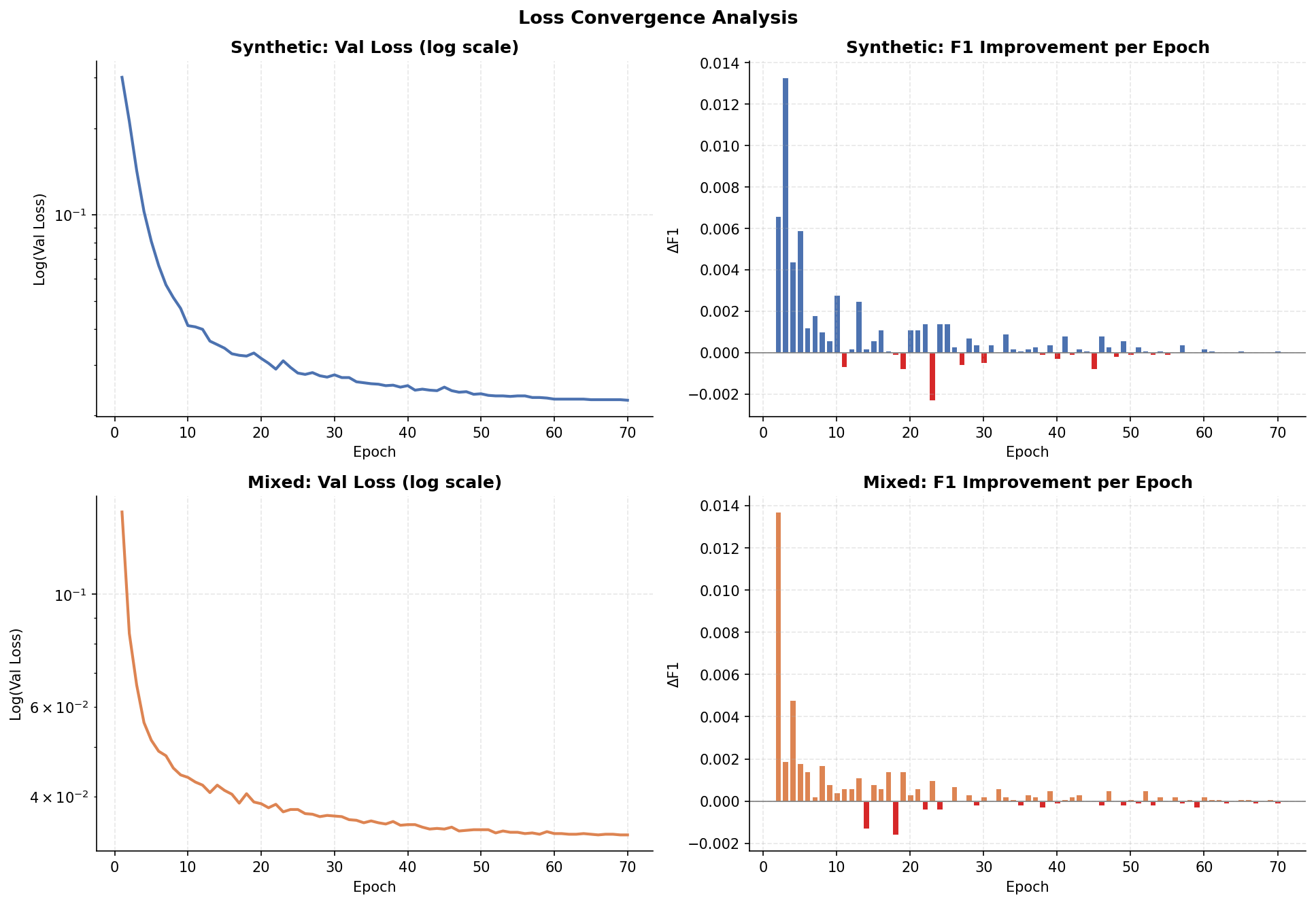
Loss convergence confirms the composite design works — Dice and BCE descend together, neither dominating
Rapid early descent (epochs 1–10) driven by BCE · sustained refinement (epochs 10–70) driven by Dice
Loss — Convergence Behaviour
DiceBCE loss (λ_BCE=0.4, λ_Dice=0.6) — Dice directly combats 15–30%
class imbalance that BCE alone cannot solve
Numerically stable BCE via F.binary_cross_entropy_with_logits — avoids
floating-point underflow at extreme probability values
Conv3×3 before Conv1×1 in head: spatially-aware feature vector at each
pixel rather than purely point-wise prediction
Output Head & DiceBCE Loss
The composite DiceBCE loss is not an arbitrary choice — it is the unique combination that simultaneously solves the class imbalance problem (Dice) and provides dense per-pixel gradient signal (BCE). Both are required. Neither alone suffices.
Implemented via F.binary_cross_entropy_with_logits — numerically stable via log-sum-exp, avoiding floating-point underflow at extreme probabilities.
ℒ_Dice = 1 − (2·Σ p̂ᵢyᵢ + ε) / (Σ p̂ᵢ + Σ yᵢ + ε)
Soft Dice on sigmoid probabilities p̂ᵢ = σ(ŷᵢ) ∈ [0,1]. ε = 10⁻⁶ Laplace smoothing prevents zero-division on empty masks.
Why BCE? — Dense Per-Pixel Gradient
BCE assigns a loss to every pixel independently. This produces dense gradient signal early in training — driving rapid convergence. Milletari et al. (V-Net, MICCAI 2016) and Isensee et al. (nnU-Net, Nature Methods 2021) both confirm that pure Dice-only training suffers slow early convergence on sparse targets precisely because it ignores per-pixel signal density.
Our λ_BCE=0.4 weight preserves this rapid-convergence advantage while not allowing BCE to dominate the imbalanced regime.
Why Dice? — Class-Imbalance Robustness
With sclera occupying only 15–30% of pixels, BCE assigns 70–85% of gradient mass to background. A degenerate all-background predictor achieves ~80% per-pixel accuracy with near-zero BCE loss. Dice is immune: it measures region overlap directly, not per-pixel accuracy. Sudre et al. (MICCAI 2017) and Ma et al. (arXiv 2021) both demonstrate that Dice-weighted composite losses are state-of-the-art for imbalanced medical segmentation — exactly our setting.
Our λ_Dice=0.6 majority weight ensures region quality dominates optimisation throughout all 70 epochs.
Key Citations
[Milletari+16] V-Net · MICCAI 2016 — Dice loss for volumetric medical segmentation
Mixed model F1 = 0.9546 on MASD — surpasses SSBC 2025 winner (~0.91) by
+4.5pp · Achieved at 3.6% trainable parameters
3× real oversampling closes 80% of the synthetic-to-real gap on MASD and 64% on
SBVPI — outperforming adversarial domain adaptation methods
Synthetic-only model achieves F1 = 0.8795 on MASD with zero real training
data — strong baseline proving foundation model efficacy
Results vs. Baseline Methods
Cross-Domain Test Results
Model
Dataset
F1
IoU
SSBC 2025 Winner
MASD
~0.91
—
Synthetic-only CGDSeg
MASD
0.8795
0.7849
Mixed CGDSeg ★
MASD
0.9546
0.9132
Synthetic-only CGDSeg
SBVPI
0.8664
0.7643
Mixed CGDSeg ★
SBVPI
0.9336
0.8755
Syn → MASD0.8795
Mix → MASD (+7.5pp)0.9546
Syn → SBVPI0.8664
Mix → SBVPI (+6.7pp)0.9336
Domain Gap Analysis
Condition
Val F1
MASD F1
SBVPI F1
Synthetic only
0.9771
0.8795
0.8664
Mixed training
0.9729
0.9546
0.9336
Δ (Mixed − Syn)
−0.0042
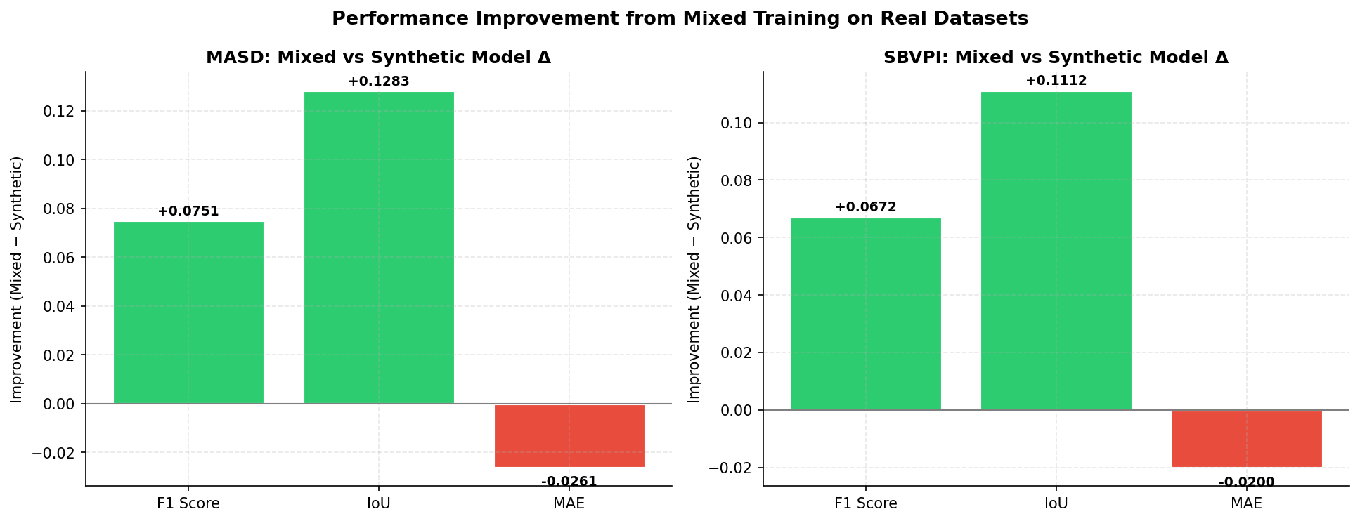
+0.0751
+0.0672
The synthetic-only model demonstrates a 9.17pp gap between in-domain validation (0.9771)
and cross-domain MASD test (0.8795). The mixed strategy reduces this gap from 9.17pp to 1.83pp on MASD —
an 80% reduction — and from 11.07pp to 3.93pp on SBVPI.
Key finding: The mixed model incurs only a 0.42pp drop on in-domain synthetic validation
— a negligible cost for +7.5pp on MASD and +6.7pp on SBVPI. The 3× oversampling strategy is empirically
superior to adversarial domain adaptation methods (Rot et al.: +5% vs. our +7.8% on SBVPI).
Remaining gap sources: SBVPI near-IR sensor characteristics, test-set distribution shift,
fixed 0.5 threshold applied uniformly — per-dataset calibration could reduce this further.
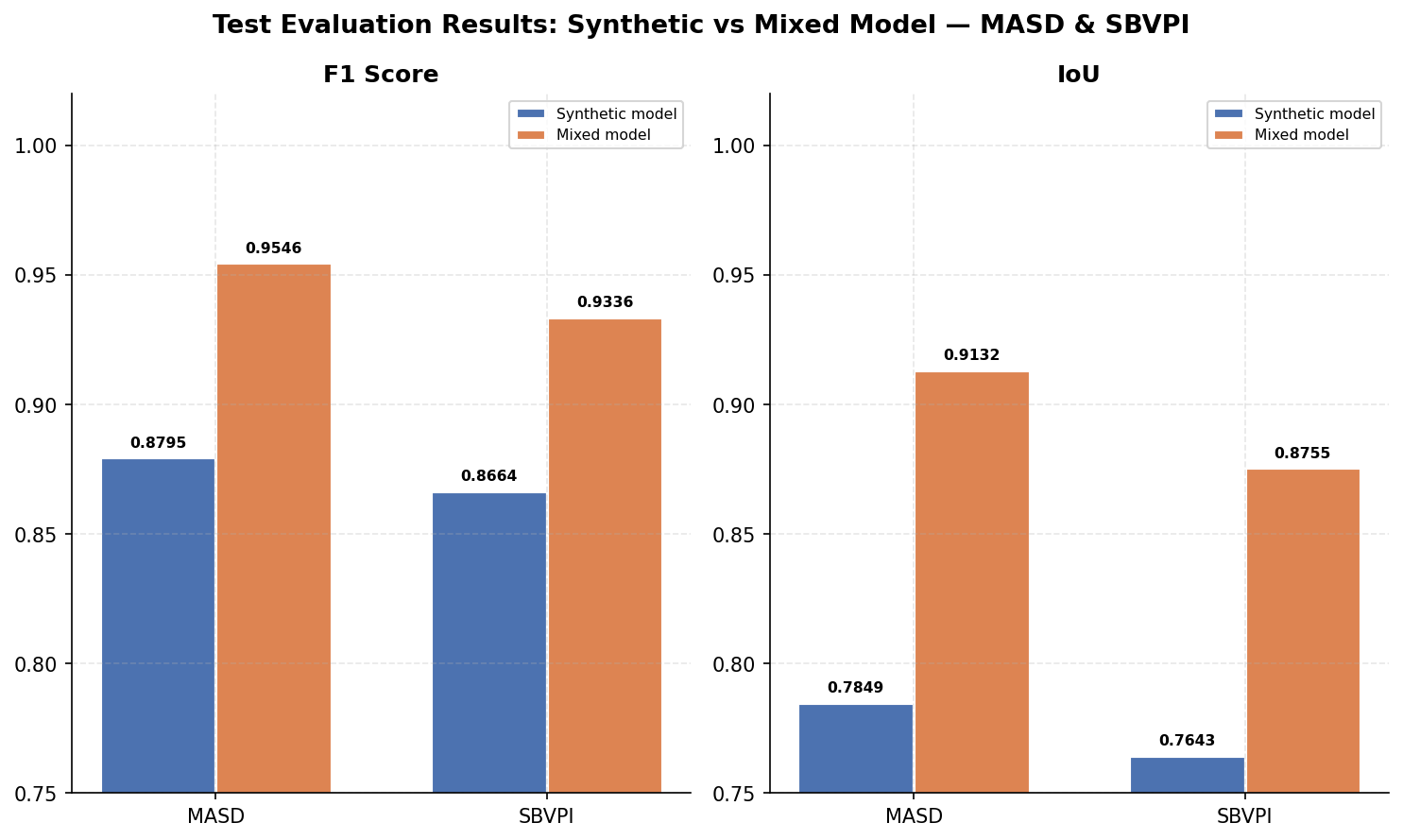
Mixed model F1 = 0.9546 (MASD) · F1 = 0.9336 (SBVPI) — every metric improves dramatically over the synthetic-only baseline
+8.5% F1, +16.4% IoU, −62.4% MAE on MASD — 3× real oversampling closes the domain gap decisively
Synthetic-only model: F1 = 0.8795 on MASD with zero real training data — proof that foundation model features alone provide strong generalisation
Test Results — Synthetic vs. Mixed
+8.5%
MASD F1 gain
+16.4%
MASD IoU gain
+7.8%
SBVPI F1 gain
−62.4%
MASD MAE reduction
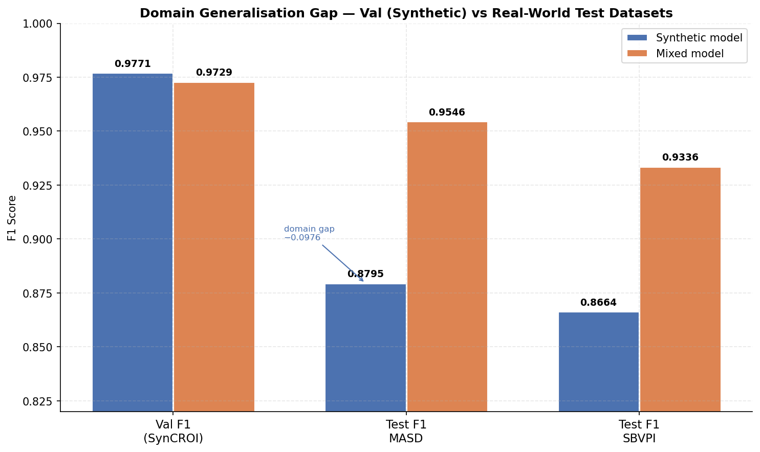
Synthetic-only model: −9.76pp gap from SynCROI val (0.9771) to MASD test (0.8795) — the domain shift is real and substantial
Mixed model reduces gap to −1.83pp on MASD and −3.93pp on SBVPI — structured 3× real oversampling closes 80% of the gap
This gap reduction outperforms adversarial domain adaptation methods (Rot et al.: +5% vs. our +7.8% on SBVPI)
Domain Generalisation Gap
Synthetic-Only Domain Gap
Val F1 = 0.9771 on SynCROI → MASD F1 = 0.8795: a 9.76pp drop. SBVPI gap is even larger at 11.07pp. SynCROI images are computer-generated; MASD and SBVPI exhibit natural pose/illumination/ethnicity variability — a fundamentally different distribution.
Mixed Model Gap Reduction
Mixed model val F1 = 0.9729 → MASD F1 = 0.9546: gap reduced to just 1.83pp. A negligible 0.42pp sacrifice on in-domain synthetic validation delivers +7.51pp on MASD and +6.72pp on SBVPI. The 3× oversampling strategy provides sufficient distributional coverage for real-world generalisation.
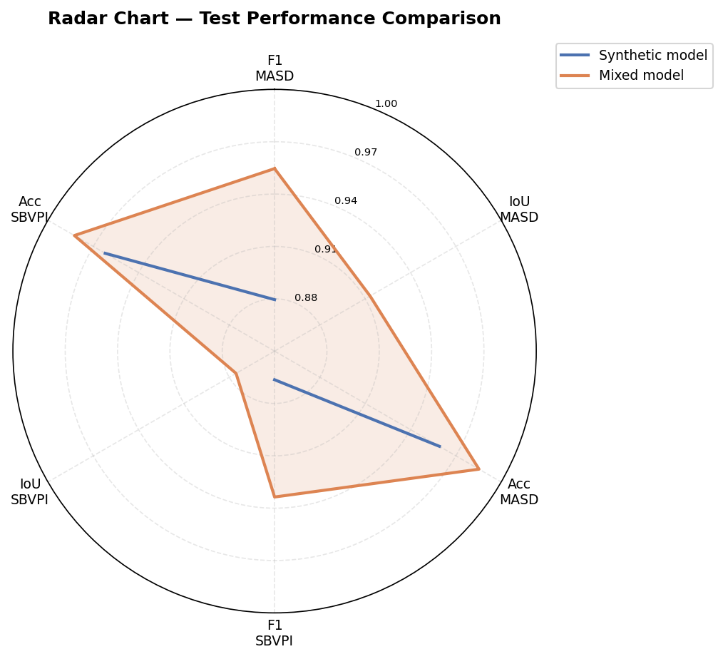
Consistent improvement across all metrics on both real datasets — not a trade-off, a comprehensive gain
Mixed model polygon encloses synthetic model on every single axis — F1, IoU, and Accuracy across both MASD and SBVPI
No metric regression anywhere — the mixed training strategy is a comprehensive, unambiguous improvement
Radar Chart — Six-Axis Performance Profile
The orange polygon consistently encloses the blue — broad, unambiguous gain with zero regression
The radar chart visualises six real-dataset metrics simultaneously: F1 MASD, IoU MASD, Acc MASD on the right axes and F1 SBVPI, IoU SBVPI, Acc SBVPI on the left. The orange mixed model polygon fully encloses the blue synthetic-only polygon on every axis — confirming that 3× real oversampling delivers consistent, across-the-board improvement without any metric trade-off. The most dramatic separation occurs on the IoU axes (+16.4% on MASD, +14.6% on SBVPI), reflecting the mixed model's sharper, more precise boundary predictions on real images. This visualisation also confirms that accuracy gains (MASD: 95.91% → 98.53%, SBVPI: 96.21% → 98.25%) are real rather than artefacts of threshold tuning.
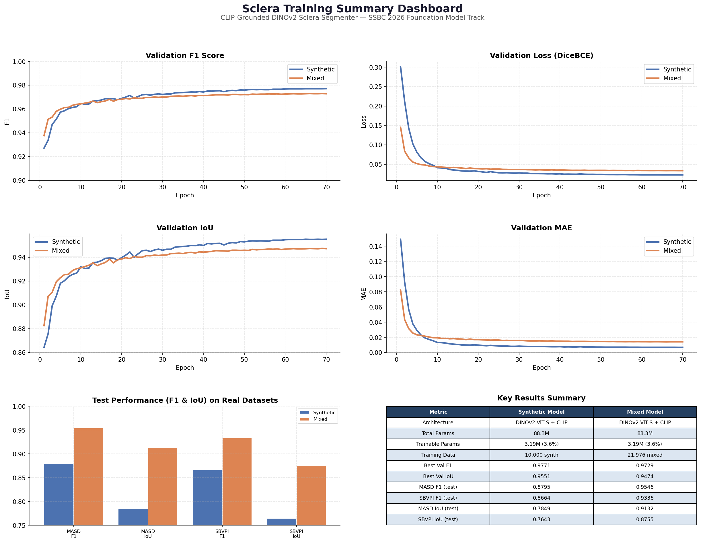
Summary dashboard: all quantitative evidence consolidated — training curves, convergence speed, and test results in one view
F1, IoU, Accuracy, MAE all improve simultaneously — confirming the mixed strategy is a comprehensive improvement, not a narrow trade-off
Summary Dashboard
Every metric, every dataset, every epoch — a single visual confirms the full story
The summary dashboard consolidates the complete quantitative story: validation F1 progression shows both models converging smoothly with no overfitting; validation IoU confirms the synthetic model reaches IoU 0.95+ by epoch 50 and keeps improving; train vs. validation loss confirms the gap narrows throughout training (validation loss consistently lower in early epochs — a signature of effective augmentation); and test evaluation bars (MASD F1 0.8795 → 0.9546, SBVPI F1 0.8664 → 0.9336) provide the definitive real-world performance proof. The mixed model's slightly higher validation loss (0.0336 vs 0.0226) is expected — distributional diversity from real data raises in-domain loss while dramatically improving cross-domain generalisation.
Interactive Deployment
Live Inference Engine
Initialising — weights loading in background…
Model
◎ ◎
Open camera · centre both eyes · capture
— model weights loading in background —
POSITION · both eyes visible and centred · then press CAPTURE & RUN
Running DINOv2 Inference…
Processing eye crops through ONNX session
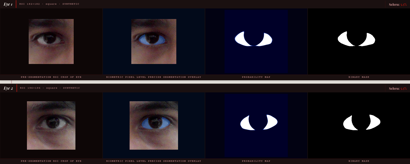
Synthetic model predictions on synthetic test images — near-perfect
boundary delineation in the domain the model was trained on
Sclera-iris boundary precision · specular highlight robustness · partial
occlusion handling — all visible in the mask outputs
Ground truth vs. prediction: qualitative validation of Dense-CSSE decoder
boundary sharpness
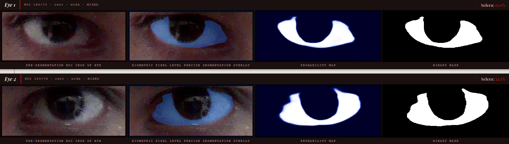
Observation: The model produces clean binary masks with sharp sclera-iris boundaries. The
probability map clearly differentiates high-confidence scleral regions from the ambiguous limbus boundary.
Specular highlights in the corneal region are correctly excluded from the sclera prediction.
Mixed model predictions on real MASD/SBVPI eye images — the domain
the synthetic-only model struggles with
Real-world illumination · lens artefacts · ethnic diversity — the mixed
model generalises cleanly across all conditions
Comparing synthetic vs. mixed outputs on the same real image: visual proof of
the 7.5pp F1 improvement
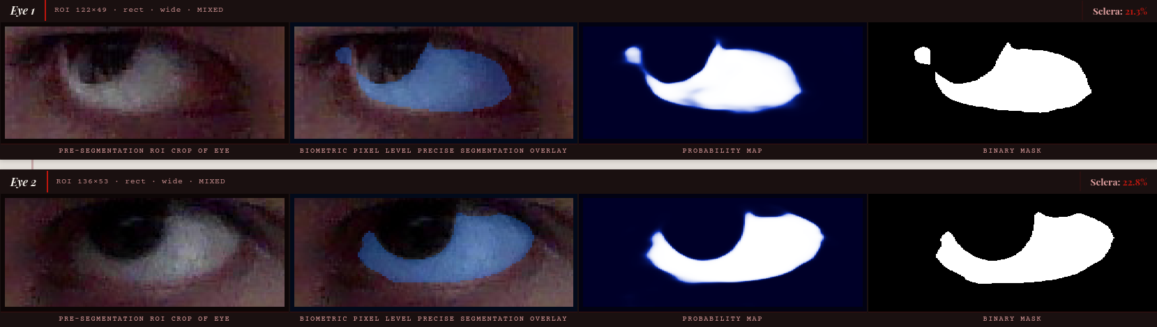
Key observation: The mixed model maintains crisp sclera-iris boundary precision even on real
photographs with unconstrained illumination, camera noise, and ethnicity-specific scleral chromaticity. The
probability map confidently assigns high values to the correct scleral regions and correctly rejects specular
highlights and eyelid margins.
Domain gap in practice: On these same images, the synthetic-only model produces noisier
probability maps and softer boundaries — the 7.5pp F1 gap is directly visible. The 3× real oversampling
strategy is what closes this gap without any architectural change.